Evolutionary Optimization of a Mathematical Function

Note

You can find the corresponding Python script here: https://github.com/Helmholtz-AI-Energy/propulate/blob/master/tutorials/propulator_example.py

The basic optimization mechanism in Propulate 🧬 is that of Darwinian evolution, i.e., beneficial traits are selected, recombined, and mutated to breed more fit individuals. Other optimizer flavors, like particle swarm optimization (PSO), covariance matrix adaptation evolution strategy (CMA-ES), and Nelder-Mead, are also available. To show you how Propulate 🧬 works, we use its basic asynchronous evolutionary optimizer to minimize two-dimensional mathematical functions. 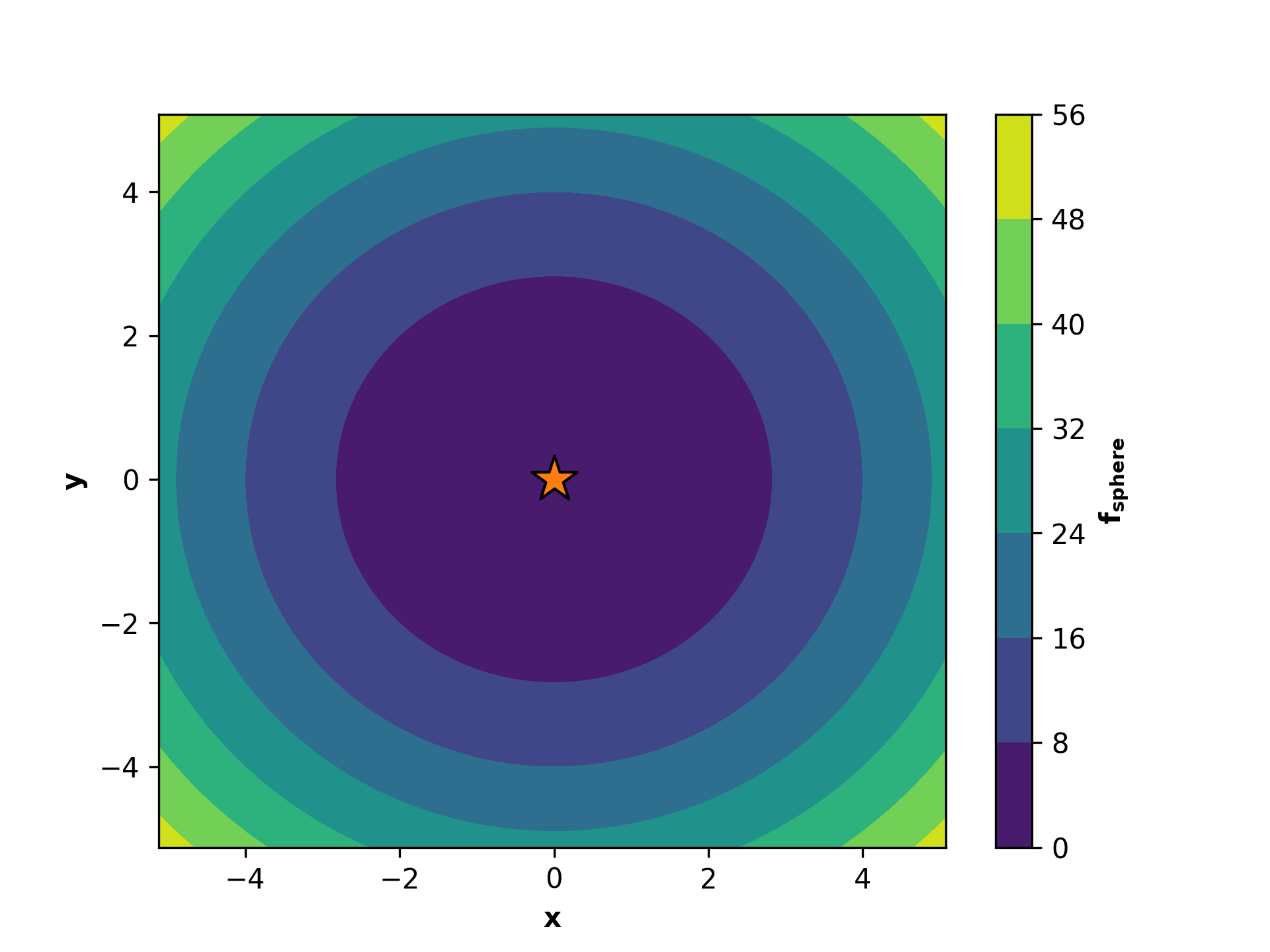Let us consider the sphere function:

\[f_\mathrm{sphere}\left(x,y\right)=x^2+y^2\]

The sphere function is smooth, unimodal, strongly convex, symmetric, and thus easy to optimize. Its global minimum is $f_\mathrm{sphere}\left(x^*=0,y^*=0\right)=0$ at the orange star.

How to Use Propulate - A Recipe

As the very first step, we need to define the key ingredients that define the optimization problem we want to solve:

The search space of the parameters to be optimized as a Python dictionary. Propulate 🧬 can handle three different parameter types:
- A tuple of float for a continuous parameter, e.g., {"learning_rate": (0.0001, 0.01)}
- A tuple of int for an ordinal parameter, e.g., {"conv_layers": (2, 10)}
- A tuple of str for a categorical parameter, e.g., {"activation": ("relu", "sigmoid", "tanh")}
Note

The boundaries for continuous and ordinal parameters are inclusive.

All-together, a search space dictionary might look like this:
```
limits = {
    "learning_rate": (0.001, 0.01),
    "conv_layers": (2, 10),
    "activation": ("relu", "sigmoid", "tanh")
}
```
The sphere function has two continuous parameters, $x$ and $y$, and we consider $x,y \in\left[-5.12, 5.12\right]$. The search space in our example thus looks like this:
```
limits = {
    "x": (-5.12, 5.12),
    "y": (-5.12, 5.12)
}
```
The fitness or loss function (also known as the objective function). This is the function we want to optimize in order to find the best parameters. It can be any Python function with the following characteristics:
- Its input is a set of parameters to be optimized as a Python dictionary.
- Its output is a scalar value (fitness or loss) that determines how good the tested parameter set is.
- It can be a black box.
Warning

Propulate 🧬 is a minimizer. If you want to maximize a fitness function, you need to choose the sign appropriately, i.e., invert your scalar fitness to a loss by multiplying it by $-1$.

In this example, the loss function whose minimum we want to find is the sphere function $f_\mathrm{sphere}\left(x,y\right)$:
```
def sphere(params: Dict[str, float]) -> float:
    """
    Sphere function: continuous, convex, separable, differentiable, unimodal.

    Input domain: -5.12 <= x, y <= 5.12
    Global minimum 0 at (x, y) = (0, 0)

    Parameters
    ----------
    params: Dict[str, float]
        The function parameters.

    Returns
    -------
    float
        The function value.
    """
    return numpy.sum(numpy.array(list(params.values())) ** 2).item()
```

Next, we need to define the evolutionary operator or propagator that we want to use to breed new individuals during the optimization process. Propulate 🧬 provides a reasonable default propagator via a utility function, get_default_propagator, that serves as a good start for the most optimization problems. You can adapt its hyperparameters, such as crossover and mutation probability, as you wish. In the example script, you can pass those hyperparameters as command-line options (this is the config in the code snippet below) or just use the default values. You also need to pass a separate random number generator that is used exclusively in the evolutionary optimization process (and not in the objective function). In addition, you can adapt the separate logger used to track the Propulate 🧬 optimization with the utility function set_logger_config as shown below:

# Set up separate logger for Propulate optimization.
propulate.set_logger_config(
    level=config.logging_level,  # Logging level
    log_file=f"{config.checkpoint}/{pathlib.Path(__file__).stem}.log",  # Logging path
    log_to_stdout=True,  # Print log on stdout.
    log_rank=False,  # Do not prepend MPI rank to logging messages.
    colors=True,  # Use colors.
)
rng = random.Random(
    config.seed + MPI.COMM_WORLD.rank
)  # Separate random number generator for optimization.
propagator = propulate.utils.get_default_propagator(  # Get default evolutionary operator.
    pop_size=config.pop_size,  # Breeding pool size
    limits=limits,  # Search-space limits
    crossover_prob=config.crossover_probability,  # Crossover probability
    mutation_prob=config.mutation_probability,  # Mutation probability
    random_init_prob=config.random_init_probability,  # Random-initialization probability
    rng=rng  # Random number generator for the optimization process
)

We also need to set up the actual evolutionary optimizer, that is a so-called Propulator instance. This will handle the parallel asynchronous optimization process for us:

propulator = Propulator(  # Set up propulator performing actual optimization.
    loss_fn=sphere,  # Loss function to minimize
    propagator=propagator,  # Evolutionary operator
    rng=rng,  # Random number generator for optimization process
    generations=config.generations,  # Number of generations
    checkpoint_path=config.checkpoint  # Checkpoint path
)

Now it’s time to run the actual optimization. Overall, generations * MPI.COMM_WORLD.size evaluations will be performed:

# Run optimization and print summary of results.
propulator.propulate(logging_interval=config.logging_int, debug=config.verbosity)
propulator.summarize(top_n=config.top_n, debug=config.verbosity)

The output looks like this:

#################################################
# PROPULATE: Parallel Propagator of Populations #
#################################################

[2024-03-12 14:37:01,374][propulate.propulator][INFO] - No valid checkpoint file given. Initializing population randomly...
[2024-03-12 14:37:01,374][propulate.propulator][INFO] - Island 0 has 4 workers.
[2024-03-12 14:37:01,374][propulate.propulator][INFO] - Island 0 Worker 0: In generation 0...
[2024-03-12 14:37:01,374][propulate.propulator][INFO] - Island 0 Worker 3: In generation 0...
[2024-03-12 14:37:01,374][propulate.propulator][INFO] - Island 0 Worker 2: In generation 0...
[2024-03-12 14:37:01,374][propulate.propulator][INFO] - Island 0 Worker 1: In generation 0...
[2024-03-12 14:37:01,377][propulate.propulator][INFO] - Island 0 Worker 3: In generation 10...
[2024-03-12 14:37:01,377][propulate.propulator][INFO] - Island 0 Worker 1: In generation 10...
[2024-03-12 14:37:01,378][propulate.propulator][INFO] - Island 0 Worker 0: In generation 10...
[2024-03-12 14:37:01,378][propulate.propulator][INFO] - Island 0 Worker 2: In generation 10...

...
[2024-03-12 14:37:02,197][propulate.propulator][INFO] - Island 0 Worker 1: In generation 960...
[2024-03-12 14:37:02,206][propulate.propulator][INFO] - Island 0 Worker 2: In generation 990...
[2024-03-12 14:37:02,206][propulate.propulator][INFO] - Island 0 Worker 1: In generation 970...
[2024-03-12 14:37:02,215][propulate.propulator][INFO] - Island 0 Worker 1: In generation 980...
[2024-03-12 14:37:02,224][propulate.propulator][INFO] - Island 0 Worker 1: In generation 990...
[2024-03-12 14:37:02,232][propulate.propulator][INFO] - OPTIMIZATION DONE.
NEXT: Final checks for incoming messages...
[2024-03-12 14:37:02,244][propulate.propulator][INFO] - ###########
# SUMMARY #
###########
Number of currently active individuals is 4000.
Expected overall number of evaluations is 4000.
[2024-03-12 14:37:03,703][propulate.propulator][INFO] - Top 1 result(s) on island 0:
(1): [{'a': '2.91E-3', 'b': '-3.05E-3'}, loss 1.78E-5, island 0, worker 0, generation 956]

Let’s Get Your Hands Dirty (At Least a Bit)

Do the following to run the example script:

Make sure you have a working MPI installation on your machine.
If you have not already done this, create a fresh virtual environment with Python: $ python3 -m venv best-venv-ever
Activate it: $ source best-venv-ever/bin/activate
Upgrade pip: $ pip install --upgrade pip
Install Propulate 🧬: $ pip install propulate
Run the example script propulator_example.py: $ mpirun --use-hwthread-cpus python propulator_example.py

Or just copy and paste:

$ python3 -m venv best-venv-ever
$ source best-venv-ever/bin/activate
$ pip install --upgrade pip
$ pip install propulate
$ mpirun --use-hwthread-cpus python propulator_example.py

Note

You can also run the script without MPI by executing $ python propulator_example.py. Both the algorithm and implementation work serially. However, this will undermine Propulate’s key feature and intended use case, i.e., asynchronous optimization for large-scale applications on supercomputers.

Checkpointing

Propulate 🧬 automatically creates checkpoints of your population in regular intervals during the optimization. You can pass the Propulator a path via its checkpoint_path argument where it should write those checkpoints to. This also is the path where it will look for existing checkpoint files to start an optimization run from. As a default, it will use your current working directory.

Warning

If you start an optimization run requesting 100 generations from a checkpoint file with 100 generations, the optimizer will return immediately.

Warning

If you start an optimization run from existing checkpoints, those checkpoints must be compatible with your current parallel computing environment. This means that if you use a checkpoint created in a setting with 20 processing elements in a different computing environment with, e.g., 10 processing elements, the behavior is undefined.

Other Optimizer Flavors

Propulate’s asynchronous communication scheme can not only be used with evolutionary algorithms but any type of population-based optimizer. In addition to Propulate’s default genetic propagator, the following alternative optimizer flavors are available, along with example scripts showing how to use them:

Covariance Matrix Adaptation Evolution Strategy (CMA-ES)

Iteratively update a population of candidate solutions using adaptive changes to the covariance matrix, guiding the search towards the optimal solution by learning the problem’s underlying structure. Here you can find a more detailed explanation of how CMA-ES works. Check out the example script for how to use CMA-ES in Propulate 🧬: https://github.com/Helmholtz-AI-Energy/propulate/blob/master/tutorials/cmaes_example.py

Two different variants of CMA-ES are available, i.e., basic [1] and active [2].

Particle Swarm Optimization (PSO)

Simulate the social behavior of birds or fish to iteratively adjust candidate solutions (particles) based on their own experience and the experience of their neighbors to find the optimal solution. Here you can find a more detailed explanation of how PSO works. Check out the example script for how to use PSO in Propulate 🧬: https://github.com/Helmholtz-AI-Energy/propulate/blob/master/tutorials/pso_example.py

Different variants of PSO are available, including basic PSO, PSO with velocity clamping, constriction PSO [3], and canonical PSO.

Nelder-Mead Optimization

Iteratively refine a simplex of candidate solutions by reflecting, expanding, contracting, and shrinking it to find the minimum or maximum of a function. Here you can find a more detailed explanation of how Nelder-Mead works. Check out the example script for how to use Nelder-Mead in Propulate 🧬: https://github.com/Helmholtz-AI-Energy/propulate/blob/master/tutorials/nm_example.py

[1] N. Hansen and A. Ostermeier (2001), “Completely Derandomized Self-Adaptation in Evolution Strategies”, Evolutionary Computation, 9(2), 159-195. https://doi.org/10.1162/106365601750190398

[2] G. A. Jastrebski and D. V. Arnold (2006, July), “Improving Evolution Strategies Through Active Covariance Matrix Adaptation”, In 2006 IEEE International Conference on Evolutionary Computation (pp. 2814-2821), IEEE. https://doi.org/10.1109/CEC.2006.1688662

[3] M. Clerc and J. Kennedy (2002). “The Particle Swarm – Explosion, Stability, and Convergence in a Multidimensional Complex Space”, IEEE transactions on Evolutionary Computation, 6(1), 58-73. https://doi.org/10.1109/4235.985692

[4] J. Kennedy and R. Eberhart, (1995, November), “Particle Swarm Optimization”, In Proceedings of ICNN’95 – International Conference on Neural Networks (Vol. 4, pp. 1942-1948). IEEE. https://doi.org/10.1109/ICNN.1995.488968